频率域滤波
使用频率域滤波器平滑图像
在频率域平滑(模糊)可通过高频的衰减来达到,即低通滤波器。本节考虑三种常用类型低通滤波器:理想滤波器、布特沃斯滤波器和高斯滤波器。所用滤波函数H(u,v)可理解为P x Q的离散函数,即离散频率变量的范围是u=0,1,2…,P-1和v=0,1,2…,Q-1。
理想低通滤波器(ILPF)

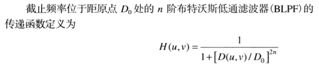
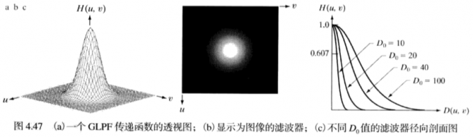
高斯滤波器(GLPF)

使用频率域滤波器锐化图像
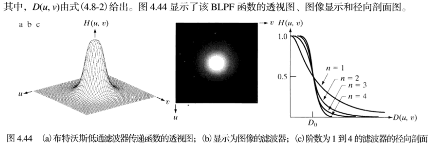
三种高通滤波器
同样是以下三种高通滤波器
频率域的拉普拉斯算子
- task4_01:
- 使用一个ILPF平滑图像。
- 使用高斯低通滤波器平滑图像。
- 使用高斯高通滤波器增强图像
- 使用拉普拉斯算子在频率域锐化图像。
代码实现:
import numpy as np
import matplotlib.pyplot as plt
from scipy import fftpack
import cv2
def high_pass_filter(img, radius=80):
r = radius
rows, cols = img.shape
center = int(rows / 2), int(cols / 2)
mask = np.ones((rows, cols, 2), np.uint8)
x, y = np.ogrid[:rows, :cols]
mask_area = (x - center[0]) ** 2 + (y - center[1]) ** 2 <= r * r
mask[mask_area] = 0
return mask
def low_pass_filter(img, radius=100):
r = radius
rows, cols = img.shape
center = int(rows / 2), int(cols / 2)
mask = np.zeros((rows, cols, 2), np.uint8)
x, y = np.ogrid[:rows, :cols]
mask_area = (x - center[0]) ** 2 + (y - center[1]) ** 2 <= r * r
mask[mask_area] = 1
return mask
def bandreject_filters(img, r_out=300, r_in=35):
rows, cols = img.shape
crow, ccol = int(rows / 2), int(cols / 2)
radius_out = r_out
radius_in = r_in
mask = np.zeros((rows, cols, 2), np.uint8)
center = [crow, ccol]
x, y = np.ogrid[:rows, :cols]
mask_area = np.logical_and(((x - center[0]) ** 2 + (y - center[1]) ** 2 >= r_in ** 2),
((x - center[0]) ** 2 + (y - center[1]) ** 2 <= r_out ** 2))
mask[mask_area] = 1
mask = 1 - mask
return mask
def guais_low_pass(img, radius=10):
rows, cols = img.shape
center = int(rows / 2), int(cols / 2)
mask = np.zeros((rows, cols, 2), np.float32)
x, y = np.ogrid[:rows, :cols]
for i in range(rows):
for j in range(cols):
distance_u_v = (i - center[0]) ** 2 + (j - center[1]) ** 2
mask[i, j] = np.exp(-0.5 * distance_u_v / (radius ** 2))
return mask
def guais_high_pass(img, radius=10):
rows, cols = img.shape
center = int(rows / 2), int(cols / 2)
mask = np.zeros((rows, cols, 2), np.float32)
x, y = np.ogrid[:rows, :cols]
for i in range(rows):
for j in range(cols):
distance_u_v = (i - center[0]) ** 2 + (j - center[1]) ** 2
mask[i, j] = 1 - np.exp(-0.5 * distance_u_v / (radius ** 2))
return mask
def laplacian_filter(img, radius=10):
rows, cols = img.shape
center = int(rows / 2), int(cols / 2)
mask = np.zeros((rows, cols, 2), np.float32)
x, y = np.ogrid[:rows, :cols]
for i in range(rows):
for j in range(cols):
distance_u_v = (i - center[0]) ** 2 + (j - center[1]) ** 2
mask[i, j] = -4 * np.pi ** 2 * distance_u_v
return mask
def log_magnitude(img):
magnitude_spectrum = 20 * np.log(cv2.magnitude(img[:, :, 0], img[:, :, 1]))
return magnitude_spectrum
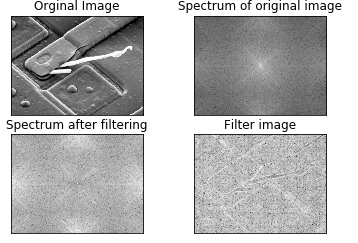
img = cv2.imread(r'D:\JupyterStore\zdip\t4_01.tif', 0)
img_dft = cv2.dft(np.float32(img), flags=cv2.DFT_COMPLEX_OUTPUT)
img_dft_shift = np.fft.fftshift(img_dft)
original_spectrum = log_magnitude(img_dft_shift)
mask = laplacian_filter(img, radius=10)
# mask = bandreject_filters(img, r_out=90, r_in=40)
# mask = high_pass_filter(img, radius=100)
# mask = low_pass_filter(img, radius=100)
# mask = guais_low_pass(img, radius=30)
# mask = guais_high_pass(img, radius=50)
fshift = img_dft_shift * mask
spectrum_after_filtering = log_magnitude(fshift)
f_ishift = np.fft.ifftshift(fshift)
img_after_filtering = cv2.idft(f_ishift)
img_after_filtering = log_magnitude(img_after_filtering)
plt.subplot(2, 2, 1), plt.imshow(img, cmap='gray')
plt.title('Orginal Image'), plt.xticks([]), plt.yticks([])
plt.subplot(2, 2, 2), plt.imshow(original_spectrum, cmap='gray')
plt.title('Spectrum of original image'), plt.xticks([]), plt.yticks([])
plt.subplot(2, 2, 3), plt.imshow(spectrum_after_filtering, cmap='gray')
plt.title('Spectrum after filtering'), plt.xticks([]), plt.yticks([])
plt.subplot(2, 2, 4), plt.imshow(img_after_filtering, cmap='gray')
plt.title('Filter image'), plt.xticks([]), plt.yticks([])
plt.show()
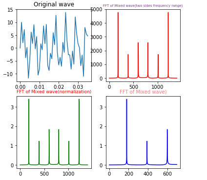
实现效果:
FFT实现
- task4_02:手工实现快速傅里叶变换。
代码实现:
import numpy as np
from scipy.fftpack import fft,ifft
import matplotlib.pyplot as plt
import seaborn
import pylab
pylab.rcParams['figure.figsize'] = (6.0,6.0)


#采样点选择1400个,因为设置的信号频率分量最高为600赫兹,根据采样定理知采样频率要大于信号频率2倍,所以这里设置采样频率为1400赫兹(即一秒内有1400个采样点,一样意思的)
x=np.linspace(0,1,1400)

#设置需要采样的信号,频率分量有180,390和600
y=7*np.sin(2*np.pi*180*x) + 2.8*np.sin(2*np.pi*390*x)+5.1*np.sin(2*np.pi*600*x)

yy=fft(y)      #快速傅里叶变换
yreal = yy.real    # 获取实数部分
yimag = yy.imag    # 获取虚数部分

yf=abs(fft(y))    # 取绝对值
yf1=abs(fft(y))/len(x)   #归一化处理
yf2 = yf1[range(int(len(x)/2))] #由于对称性,只取一半区间

xf = np.arange(len(y))  # 频率
xf1 = xf
xf2 = xf[range(int(len(x)/2))] #取一半区间


plt.subplot(221)
plt.plot(x[0:50],y[0:50])
plt.title('Original wave')

plt.subplot(222)
plt.plot(xf,yf,'r')
plt.title('FFT of Mixed wave(two sides frequency range)',fontsize=7,color='#7A378B') #注意这里的颜色可以查询颜色代码表

plt.subplot(223)
plt.plot(xf1,yf1,'g')
plt.title('FFT of Mixed wave(normalization)',fontsize=9,color='r')

plt.subplot(224)
plt.plot(xf2,yf2,'b')
plt.title('FFT of Mixed wave)',fontsize=10,color='#F08080')


plt.show()
实现效果: